📚 Introduction
This is the introduction to a series on Abstract Algebra. In particular, our focus will be on Galois Fields (also known as Finite Fields) and their applications in Computer Science.
Backstory
Many moons back I was self-learning Galois Fields for some erasure coding theory applications. I was quite disappointed with the lack of accessible resources for computer scientists. Many resources assume either:
- It's beyond your skill level, so let's oversimplify ("it's hard, don't worry about it"), or
- You had prior Pure Math studies in Abstract Algebra ("it's easy, just use jargon jargon jargon")
Unfortunately, Abstract Algebra is not standard subject matter in most computer science curriculums. Often computer science mathematics start and end with Discrete Math. If you're lucky, maybe you've also been exposed to Linear Algebra.
So, ultimately, I ended up self-learning Abstract Algebra from a pure math textbook. But for the great majority of computer scientists, there has to be a better way. This series intends to fill this gap. This is the gentle step-by-step approach with applications implemented with actual code. It's the intro you wanted when you were starting out.
What is this subject?
Abstract algebra is a beautiful subject. It's the idea that the numbers you're familiar with don't matter. The numbers are just arbitrary labels. What matters is the relationships they have with other numbers when you add or multiply them. If the numbers don't matter, then we can swap those labels for different labels and all the normal math rules will still work.
For example, we could create an algebra that allows us to add or multiply colors:
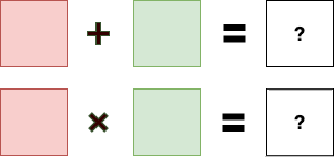
And this is what makes the subject abstract and confusing. How can you just say that numbers don't matter? It doesn't make sense.
And even so, why would we want to study this? Why would a computer scientist care?
Well, we use computer algorithms to manipulate data. We encode/decode it, we encrypt/decrypt it, we detect corruption, etc. Wouldn't it be great if we could use normal math to do those things? Wouldn't it be great if we could add or multiply an 8-bit byte by an 8-bit byte and get another 8-bit byte?
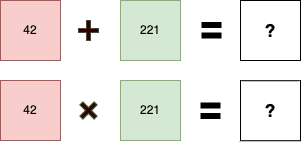
(Hint: Neither 263 nor 9282 are answers, they are not 8-bit numbers)
And if we could do that, could we also do Linear Algebra over Data? Yes, yes, and more yes. This is why studying Abstract Algebra is worthwhile.
You can also make quirky blog posts that make your friends think you've gone crazy, like milk and cookie 🥛 🍪 😊
Applications
The applications and algorithms are staggering. You interact with implementations of abstract algebra everyday:
- CRC (Cyclic Redundancy Check) — error detection in network protocols
- AES Encryption — the Advanced Encryption Standard uses GF(2⁸)
- Elliptic-Curve Cryptography — modern public-key cryptography
- Reed-Solomon — error correction in CDs, QR codes, RAID systems
- Advanced Erasure Codes — distributed storage systems
- Data Hashing/Fingerprinting — efficient data identification
- Zero-Knowledge Proofs — cryptographic proofs without revealing secrets
Having a solid background in Galois Fields and Abstract Algebra is a prerequisite for understanding these applications.
Approach: Step-by-step, Active Learning, and Literate Programming
In this series, we will start from the very basics of theory and build up step-by-step to interesting applications such as Reed-Solomon, AES, etc. As such, the material will be very cumulative. Many exercises will be included to aid understanding. Each section will build gradually, but will assume mastery of the previous section. Active learning is strongly encouraged.
We won't assume too much mathematical background beyond high-school level algebra. However, in some applications (for example: Reed-Solomon), familiarity with Linear Algebra will be required. We won't assume you know Linear Algebra, but we will introduce it here when needed.
We will be including code in a Literate Programming style where appropriate. For example, to aid understanding, we will build some interactive command-line tools that allow you to play around with various operations. The code will be written in the Rust Programming Language.
The main goal of this series is understandability and education. As such, the implementations will not be optimal. We will forgo nearly all optimizations you'd see in a production quality implementation.
For active learning, I strongly encourage you to do your own implementations and to play around with the command-line tools while reading. If you'd like to open-source your implementation, I'm more than happy to link to it.
- Original: xorvoid (Rust): here
Planning is Essential, Plans are Worthless
Here's the rough plan. We will see how it actually goes:
- Group Theory
- Field Theory
- Implementing GF(p)
- Polynomial Arithmetic
- Polynomial Fields GF(p^k)
- Implementing GF(p^k)
- Implementing Binary Fields GF(2^k)
- Cyclic Redundancy Check (CRC)
- Linear Algebra over Fields
- Reed-Solomon as Polynomial Representation
- Reed-Solomon as Linear Algebra
- AES (Rijndael) Encryption
- ... And More ...
Other possible advanced subjects:
- Rabin Fingerprinting
- Extended Euclidean Algorithm
- Log and Invlog Tables
- Elliptic Curve
- Bit-matrix Representation
- Fast Multiplication with FFT
- Vectorization Implementation Techniques
The first few sections are theory. There's not much coding in these sections, but they are very important for success later in the series. Don't skip them.
🔢 Group Theory
This is part 1 of a series on Abstract Algebra. In this part, we'll give a gentle introduction to Group Theory.
Clock Arithmetic
A Group is one of the basic algebraic structures studied in Abstract Algebra. It's simply a set of "numbers" and an "operation" on them. The operation is normally referred to as "addition" or "multiplication", but it doesn't have to be.
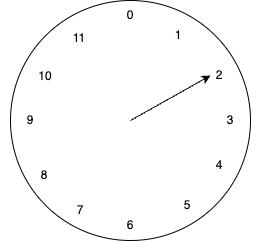
In fact, you are already very familiar with a Group: A Clock.
Of course, as computer scientists, we must start our numbers at 0 because we're all neurodivergent and we take great pleasure in annoying mathematicians.
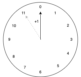
Our clock uses the numbers {0, 1, 2, 3, 4, 5, 6, 7, 8, 9, 10, 11} and has the operation of "an hour passes". If the hour-hand points to 2 and the "operation" occurs, it now points at 3.
Similarly, if it points at 11, then after the "operation" it will point to 0 (roll over to the beginning).
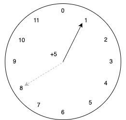
Or we can "add" 5 hours to 8 and we will get 1.
Or we can "add" 0 hours and the hour will stay the same!
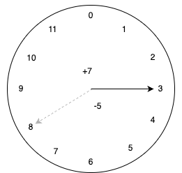
We can even "subtract", which is going backwards around the clock. Subtracting 5 hours from 8 gives 3. Just like arithmetic over integers, subtraction is just addition in disguise. We just add the "negative" or "inverse" of 5.
In short, we can do all of the following on this clock:
- We can add n hours to any position, yielding a new position on the clock
- We can find an additive-inverse of any position that can convert any subtraction into an addition
- We can add zero and the position doesn't change
- We can do associative addition, i.e. (1 + 2) + 3 = 1 + (2 + 3)
Here are some examples of operations on our clock:
| Operation | Result |
|---|---|
| 0 + 1 | 1 |
| 5 + 3 | 8 |
| 8 + 5 | 1 |
| 11 + 1 | 0 |
| 7 + 0 | 7 |
| 3 - 5 | 10 |
| (2 + 3) + 4 | 9 |
| 2 + (3 + 4) | 9 |
Practice: Clock Addition
Practice: Clock Subtraction
Practice: Additive Inverse
Group Definition
The clock example we gave above is an example of a Group. It's helpful to keep the example in mind as we start introducing abstract definitions.
A Group is defined as some operation ( + ) defined over a set of "numbers" which follow these rules:
- Associativity: (a + b) + c = a + (b + c)
- Identity: one of the numbers acts like a "zero": a + e = a, e + a = a
- Inverse: each element a has some unique element b where a + b = e
And that's it.
The name of the operation isn't important. Sometimes we use the multiplication ( * ) operator instead. The notation doesn't matter.
Modular Arithmetic
Our clock arithmetic group is an example of Modular Arithmetic. In particular, it's the special case where modulus n = 12. There's no special reason we need to use 12. We can use any modulus n we want. For example, we could have a 5-hour clock, or a 7-hour clock, etc.
In modular arithmetic, the following notation is commonly used:
a ≡ b (mod n)
This says that a and b are logically the same value when using modulus n. Consider our clock again, if the hour hand points at 5 and we add 12 hours, we'd be at 17 right? But we don't have a 17 hour on our clock. So we wrap around and we're back at 5.
In modular arithmetic notation, we'd express this as:
5 ≡ 17 (mod 12)
Similarly there are an infinite number of integers that are "equivalent" to 5 when modulus n=12:
5 ≡ 17 ≡ 29 ≡ 41 ≡ ... (mod 12)
In general:
a ≡ b (mod n) if and only if (a - b) is divisible by n
In this way, we can think of modular arithmetic as doing normal arithmetic and then only keeping the remainder after applying the modulus.
Do the exercise. Each section gets harder. You need to fully understand each or you'll get lost later.
Modular Arithmetic: Multiplication
How about the same modular arithmetic, but with multiplication instead of addition? Let's see...
We want to do:
a * b (mod n)
Examples with our n=12 clock:
- 2 * 3 = 6 (mod 12)
- 4 * 5 = 20 ≡ 8 (mod 12)
- 3 * 4 = 12 ≡ 0 (mod 12)
Don't read on before completing the exercise.
Click to reveal answer
First, it's clear that 1 must be the identity element because:
a * 1 = a, 1 * a = a
We need a multiplicative inverse for each element, including 0:
0 * x = 1 (mod 12)
But, there's no solution! So the set {0, 1, 2, 3, 4, 5, 6, 7, 8, 9, 10, 11} is not a group using multiplication.
What if we just get rid of 0 then and use the subset {1, 2, 3, 4, 5, 6, 7, 8, 9, 10, 11}?
Is this a group now? Unfortunately no. Not every element has an "inverse".
Consider the element 2. We need to find some x such that: 2 * x = 1 (mod 12).
Exercise: Try each of the numbers {1, 2, 3, 4, 5, 6, 7, 8, 9, 10, 11} for x to try solving 2 * x = 1 (mod 12). Is there an inverse for 2? Can you think of simple reason why not?
So maybe modular arithmetic doesn't work? Give Up? Actually no.
Modular arithmetic over multiplication works if the modulus n is prime. This is a direct result of important facts in number theory involving the Greatest Common Denominator and Bezout's Identity.
Proof (you can skip this):
Let a be some number from the set of numbers in our Group. And suppose we wish to find an inverse b such that:
a * b ≡ 1 (mod n)
We'll rearrange this expression:
a * b - 1 = k * n (for some integer k)
We've achieved a form where we can use an important identity.
Bezout's Identity states that given x and y, we can always solve for a and b in the equation:
gcd(x, y) = a*x + b*y
So we can solve:
gcd(a, n) = a*x + n*y
And b will be our desired inverse when:
gcd(a, n) = 1
When n is prime, we have gcd(a, n) = 1 always (for a in {1, 2, ..., n-1}). So we must always have a solution.
The proof is complete.
With this result we can satisfy our 3 group properties and conclude that modular-arithmetic over the set {1, 2, ..., p-1} is always a group when p is prime.
Next Step
You should be very comfortable with this material before moving on. If you aren't, go back and do more examples. Perhaps draw some clocks with different number of hours and see what happens? This is a critical foundation.
Next up, we will extend Group Theory into Field Theory.
⚡ Field Theory
This is part 2 of a series on Abstract Algebra. In this part, we'll extend the idea of a Group into the idea of a Field.
Where we're going
To build a Field, we're basically going to glue two groups together. Something like gluing a car and truck together.
Now, I know what you're thinking: "Hey, they tried that in 60s and it was weird..."

I hear what you're saying, but this is not a Design By Committee blog post, okay... That ends in weird car designs also. My blog, my rules.
Our goal is to glue a Car group and Truck group together and NOT get an El Camino.
Vehicles and Glue
We're going to combine the main two groups we discussed last time into a single unified field. We built an addition group and a multiplication group last time. For multiplication we need a prime-number modulus.
Visually:
| Group | Operation | Set | Modulus |
|---|---|---|---|
| Addition Group | + | {0, 1, 2, ..., p-1} | p (any integer) |
| Multiplication Group | * | {1, 2, ..., p-1} | p (must be prime) |
Uh oh. Big problem: Zero doesn't behave correctly in a multiplication group!
We said at the beginning that finite fields are like normal math with weird numbers. In normal math, zero is also weird. So weird that it took mathematics a long time to accept it (which is another reason why we start at 0 as computer scientists).
Our workaround will be the same as in normal math. Our numbers will be {0, 1, 2, 3, ..., p-1} and we'll define 0 * a = 0 for all numbers a. And for multiplicative inverses and division with zero... umm... we just don't do that. Division by zero is undefined, just like in normal math.
Congratulations: We've constructed GF(p)!
Before proceeding, I want to explain this notation. GF stands for Galois Field which is just a synonym for Finite Field named after Évariste Galois who had a short-lived but fascinating life (wiki).
Exploring GF(5)
Let's make this more concrete by exploring GF(5). First, this notation tells us there are 5 numbers in this field. Let's denote them as {0, 1, 2, 3, 4}.
Addition in this field is just plain modular-arithmetic addition:
| + | 0 | 1 | 2 | 3 | 4 |
|---|---|---|---|---|---|
| 0 | 0 | 1 | 2 | 3 | 4 |
| 1 | 1 | 2 | 3 | 4 | 0 |
| 2 | 2 | 3 | 4 | 0 | 1 |
| 3 | 3 | 4 | 0 | 1 | 2 |
| 4 | 4 | 0 | 1 | 2 | 3 |
Multiplication is similar, with the quirk about 0:
| * | 0 | 1 | 2 | 3 | 4 |
|---|---|---|---|---|---|
| 0 | 0 | 0 | 0 | 0 | 0 |
| 1 | 0 | 1 | 2 | 3 | 4 |
| 2 | 0 | 2 | 4 | 1 | 3 |
| 3 | 0 | 3 | 1 | 4 | 2 |
| 4 | 0 | 4 | 3 | 2 | 1 |
Additive inverses:
| Element | Additive Inverse |
|---|---|
| 0 | 0 |
| 1 | 4 |
| 2 | 3 |
| 3 | 2 |
| 4 | 1 |
Multiplicative inverses:
| Element | Multiplicative Inverse |
|---|---|
| 1 | 1 |
| 2 | 3 |
| 3 | 2 |
| 4 | 4 |
Finally, let's demonstrate an important property of a field.
Consider 4*(2+1) and (4*2) + (4*1). Are these equal?
Yes! Does this work in general? Also, yes.
The distributive property holds for fields:
a * (b + c) = (a * b) + (a * c)
Definition
We're now ready to be math lawyers and go all definitional.
A Field is defined as two operations ( + and * ) defined over a set of "numbers" which follow these rules:
- Associativity: (a + b) + c = a + (b + c), (a * b) * c = a * (b * c)
- Commutativity: a + b = b + a, a * b = b * a
- Identity: An additive identity ( 0 ) and a multiplicative identity ( 1 ) where: a + 0 = a, a * 1 = a
- Additive inverse: for each a there is some b such that a + b = 0
- Multiplicative inverse: for each a != 0 there is some b such that a * b = 1
- Distributivity: a * (b + c) = (a * b) + (a * c)
And that's it. You now know what a field is.
This is effectively just formalizing up what is usual and common in the Real Numbers. This is why I say "it just works".
I need to however say one note on "commutativity". Our definition of groups did not require commutativity. This is common in group definitions. But the addition and multiplication groups used in a field are commutative. There are non-commutative groups (like permutation groups or Matrix Multiplication Group GL(n,R)), but we won't be using those.
Finally, the definition of Field is very general and says nothing about the size. We can have infinite sized Fields. For example, the Real Numbers are a Field. The Rational Numbers are also a field.
The Lonely Misfit
We're skipping a very large amount of the standard Abstract Algebra treatment in this series. We're just plucking out the parts that are directly useful to finite-fields. There is a very large and interesting subject here that we're not covering. If you're interested, I'd recommend checking out a proper Abstract Algebra textbook. For now, we're just going to focus on what we need.
Next Step
You should be very comfortable with this material before moving on. If you aren't, go back and do more examples. This is a very cumulative subject and in each section, I will assume you've mastered the previous sections.
If you follow everything so far, congrats. You're rockin' math: Time to Celebrate!
Next up, we'll finally begin coding, starting with a GF(p) implementation!
🔐 GF(p) - Prime Fields
This is part 3 of a series on Abstract Algebra. In this part, we'll implement the GF(p) fields we discussed last time.
Implementing GF(p)
Source Code: src/gf_p.rs
An implementation of GF(p) where p is a prime number
We will implement addition, subtraction, multiplication, and division using operator-overloading so we can use the normal operators: +, -, *, /
use std::ops::{Add, Mul, Sub, Div};
Rust supports Const Generics, but that adds a lot of extra syntax noise which may be distracting for readers without a background in Rust or C++.
Instead, we'll just define a simple constant. If you'd like to explore a GF(p) field for a
different prime, just change the number below. You are responsible for ensuring that the number is actually
prime. By default, we'll use GF(5):
pub const P: u8 = 5;
The type we use to represent a number in GF(p) is just an unsigned 8-bit integer (u8).
This design will allow for prime fields up to size 251 (the largest prime that fits
in 8-bits). We will also tell Rust that its okay to copy (Clone & Copy) and to compare
two numbers via equality (PartialEq)
#[derive(Debug, Clone, Copy, PartialEq)]
pub struct GF(u8);
Constructing a new number in GF(p) is easy: we just need to ensure it's within
the set {0, 1, ..., p-1}
impl GF {
  pub fn new(val: u8) -> GF {
    assert!(val < P);
    GF(val)
  }
  pub fn value(&self) -> u8 {
    self.0
  }
}
Addition and Subtraction
Now we implement addition via simple modular arithmetic: (a + b) % p.
But we need to take care to avoid 8-bit overflow, so we do the math in
16-bit (u16) and then apply the modulus operation.
impl Add<GF> for GF {
  type Output = GF;
  fn add(self, rhs: GF) -> GF {
    let a = self.0 as u16;
    let b = rhs.0 as u16;
    let p = P as u16;
    GF::new(((a + b) % p) as u8)
  }
}
Negation (or additive-inverse) is fairly straight-forward also.
Given a, we want to solve for neg(a) in:
a + neg(a) == 0 (mod p)
It seems like the answer would be:
neg(a) = p - a
But if a == 0, then we'd compute neg(a) = p which is not a valid number.
This has an easy fix though:
neg(a) = (p - a) % p
impl GF {
  pub fn negate(self) -> GF {
    GF::new((P - self.0) % P)
  }
}
Now, we can easily implement subtraction in terms of addition and negation
since: a - b = a + (-b)
impl Sub<GF> for GF {
  type Output = GF;
  fn sub(self, rhs: GF) -> GF {
    self + rhs.negate()
  }
}
Multiplication and Division
Now we implement multiplication via simple modular arithmetic: (a * b) % p.
But we need to take care to avoid 8-bit overflow, so we do the math in
16-bit (u16) and then apply the modulus operation.
impl Mul<GF> for GF {
  type Output = GF;
  fn mul(self, rhs: GF) -> GF {
    let a = self.0 as u16;
    let b = rhs.0 as u16;
    let p = P as u16;
    GF::new(((a * b) % p) as u8)
  }
}
Multiplicative inverses are the trickiest operation in this field. We will implement them by brute force. If we've constructed a proper field, then each number will have an inverse. If we try all numbers, one will succeed.
Notice the Result<> type here. This is Rust's way of returning errors. We need to
use a Result<> here since the number 0 has no inverse and need to communicate that
the operation has failed.
Faster approaches exist (e.g. The Extended Euclidean Algorithm), but for a first implementation we will avoid adding that complexity. We'll discuss faster methods in later sections.
impl GF {
  pub fn invert(self) -> Result<GF, String> {
    // Important: Zero has no inverse, it's invalid
    if self.0 == 0 {
      return Err("Zero has no inverse".to_string());
    }
    // Scan the numbers {1, 2, ..., P-1} until we find the inverse
    for x in 1..P {
      let candidate = GF::new(x);
      if self * candidate == GF::new(1) {
        return Ok(candidate); // Found!
      }
    }
    unreachable!("Every non-zero number has an inverse");
  }
}
Similarly to subtraction, we can implement division in terms of multiplication
and inversion since: a / b = a * inv(b)
Notice that division by zero panics (crashes). We expect the user to avoid attempting a divide by zero.
impl Div<GF> for GF {
  type Output = GF;
  fn div(self, rhs: Self) -> GF {
    // Important: Cannot divide by zero
    if rhs.0 == 0 {
      panic!("Cannot divide by zero");
    }
    self * rhs.invert().unwrap()
  }
}
Some final things
Rust as a language doesn't implicitly assume much about new types so we have to explicitly tell it how to do a few more-or-less trivial things.
We need to tell Rust how to print these new numbers to the screen. We will just print them out as ordinary integers.
impl std::fmt::Display for GF {
  fn fmt(&self, f: &mut std::fmt::Formatter) -> std::fmt::Result {
    write!(f, "{}", self.0)
  }
}
And, we need to tell Rust how to convert strings into our field's numbers.
impl std::str::FromStr for GF {
  type Err = String;
  fn from_str(s: &str) -> Result<GF, String> {
    let num: u8 = s.parse().map_err(|_| format!("Not an 8-bit integer"))?;
    // Return an error if the number is too big for the field
    if num >= P {
      return Err(format!("Number too large, got {}, but limit is {}", num, P-1));
    }
    Ok(GF::new(num))
  }
}
Finally, we'll tell rust that that our implementation can be treated as a Field in any code that is written for Fields! This will come in handy for our calculator.
impl crate::field::Field for GF {
  fn number_of_elements() -> usize {
    P as usize
  }
}
Testing Time
Note that these tests assume GF(5). If you change the size of the field, they are not expected to pass.
Exercise: Play around with the calculator. Change P to a different prime and explore that field too.
Exercise: Do your own implementation of GF(p) fields in your preferred programming language.
Next Up
Hopefully this section helps put a lot of pieces together.
Is it a little weird that 2*4 = 3? Maybe.
But that's why I say that the numbers are weird but everything just works like normal. It's a Field because it behaves like a Field. And, that's all we care about in Abstract Algebra.
The work we've done so far is already quite useful, but for computing, this restriction to prime numbers is awkward. We really want fields like GF(4), GF(16), GF(64), GF(256), etc that map well to binary data.
To do this we'll need more abstraction and get reacquainted with an old friend: Polynomial
📊 Polynomial Arithmetic
Content coming soon...
🌐 GF(p^k) - Extension Fields
Content coming soon...
⚙️ GF(2^k) - Binary Fields
Content coming soon...
📐 Linear Algebra over Fields
This is part 9 of a series on Abstract Algebra. In this part, we'll start doing Linear Algebra over Finite Fields.
Content will be inserted here...
📈 Reed-Solomon as Polynomial Representation
This is part 10 of a series on Abstract Algebra. In this part, we'll start exploring Reed-Solomon Erasure Codes.
Content will be inserted here...
🔬 Reed-Solomon as Linear Algebra
This is part 11 of a series on Abstract Algebra. In this part, we'll continue exploring Reed-Solomon Erasure Codes.
Content will be inserted here...